Revamping Airline Demand Forecasting
Take Our Content to Go
Airline Industry Forecasting
In the airline industry, it is valuable for management to know ahead of time how many seats will likely be occupied on any given flight. Because the number of seats booked affects resourcing demands and revenue, knowledge of booking trends can help airlines plan ahead. Traditionally, data scientists have approached this forecasting problem from two standpoints: backward—looking for trends in historical data for departed flights to inform predictions of future bookings, or forward—looking at bookings that have already been made for a future departure date to predict future demand. The results of these two approaches are also sometimes blended together as a combined model to make the final forecast.
Historical Booking Model
The historical booking model looks at final bookings (reservations) for a particular flight from a historical perspective. Data scientists study past final bookings data, identify seasonal variations and cyclical trends, and use this behavior to predict their future behavior.
The historical booking model uses various algorithms to forecast final bookings for a particular flight on a particular day (or week or month) in the future. Various approaches may be used to obtain a forecast result, including moving averages, exponential smoothing (including Holt-Winters), ARIMA time-series forecasting, and linear regression. Interestingly, one study has demonstrated that more complex methods such as ARIMA rarely outperform simpler ones.1
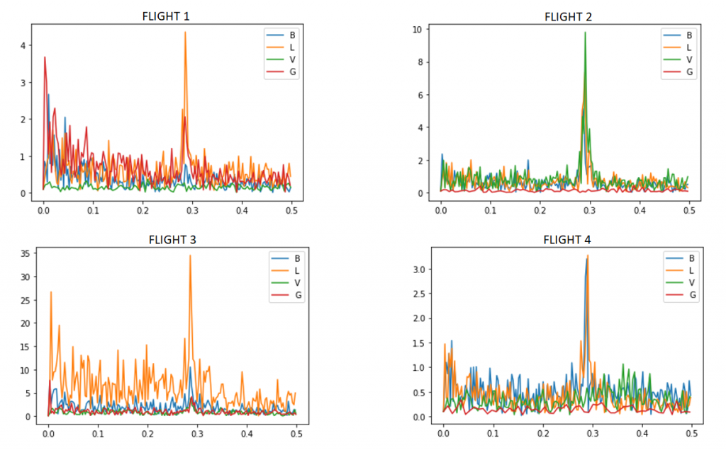
Regardless of the algorithm used, all approaches try to capture seasonal and cyclical characteristics from the historical data. The graphs shown in Figure 1 below illustrate this phenomenon through spectral analysis, achieved by applying a Fast Fourier Transform (FFT) to the time-series booking data for four different flights. The spikes at roughly 0.3 on the x-axis (frequency) reflect weekly cycles, i.e., similar demand for the same day of the week. The spikes near 0.0 on the x-axis for Flights 1 and 3 on the left-hand side reflect seasonal/annual patterns not exhibited by Flights 2 and 4 on the right-hand side. Finally, the different colors represent different fare/customer categories. It is readily apparent that each flight has a unique clientele; moreover, the behavior of customer types varies across different flights.
Advance Booking Model
While the historical booking model aims to learn from past results and extrapolate to the future, the advance booking model uses the nature of airline reservations themselves—i.e., that they are typically made in advance—to predict the demand on a given day. The advance booking model looks at the cumulative bookings for a particular future flight as they come in. Because these dates are in the future, the booking data does not reveal the final seats that will be bought. To predict how many more reservations will be made for the departure date in question, the advance booking model uses the “on the book” demand for the days before departure.
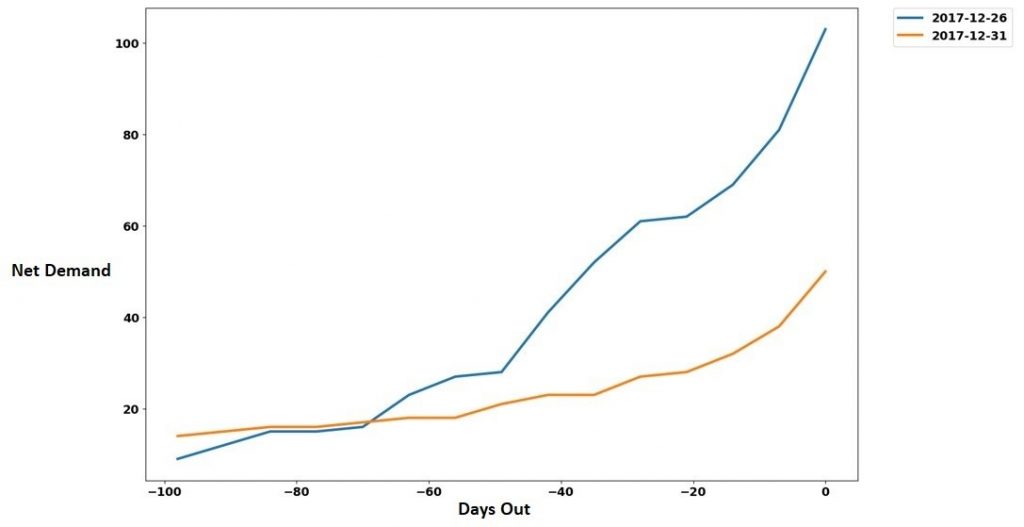
The core of this approach is a technique called a booking curve, which shows the cumulative advance bookings made as you get closer to the date of departure. Figure 2 depicts the booking curve for two sample departure dates for the same flight. As you can see on the far left of the graph, not many seats have been booked more than 100 days out from the two sample departure dates. The number of bookings increases up until and including the date of departure itself (where it sometimes can take a small dip due to last-minute cancellations).
Combining Models
There are trade-offs to consider in the two forecasting models described above. For example, while the advance booking model is typically more accurate than the historical booking model because it has new information in the form of actual reservations for the flight of interest, the advance booking model cannot extend as far back in time. At 365 days out, a flight typically has no reservations yet, so using the booking curve is no better than simply predicting that the same number of seats will be occupied at the future date as the same day the previous year. However, the two models described can be blended in such a way as to exploit each model’s strengths and compensate for its weaknesses.
The general approach to blending the models is to weight the two forecasts according to how far out you are from the departure date. Thus, a prediction for a departure date a year from now would rely almost exclusively upon the historical booking model, while a prediction for a departure next week would rely heavily upon the advance booking model. The weighting approach can vary, but is not linear (i.e., giving equal weight 6 months out) because the advance booking model usually comes into play within 120 days of a flight.
Innovating on Industry Norms: Prophet and Mathematical Tuning
In a prior project, Mosaic, an innovative airline data analytics consulting company, approached the demand forecasting challenge using the historical booking model and the advance booking model. We began our work on the historical booking model in the same way we would begin work on any other machine learning (ML) modeling problem: by testing various features and ML algorithms. Because almost all the information comes from time-series features (day of week, month, week of year, holidays, etc.), appropriate time-series methods needed to be applied. The challenge is that airlines may only have a few years of data to train a predictive model on, which could mean only one year of holdout data would be available for testing and validation. Given the limited data, Mosaic’s data science consultants were able to gain additional performance over traditional methods by including segmentation at the fare class level and then aggregating the results. The Mosaic data science team developed models for each flight independently and evaluated generalized linear models, random forest, and XGBoost. After proper tuning, XGBoost was found to outperform the others significantly.
Unfortunately, XGBoost took a significant amount to time to train each model due to hyperparameter tuning. At roughly 12 minutes per flight, this would not scale well to thousands of flights, requiring more than a hundred hours per training run. So, in search of greater performance and decreased training time, the team decided to try Prophet, a time-series forecasting tool recently open-sourced by Facebook (and available in packages for both R and Python). Using Prophet, Mosaic data science consultants were able to get as good or better performance as with XGBoost, and at the same time decrease training time to under a minute per flight.
For flights that were consistently booked close to the seat capacity of the airplane, the team performed a log transform of the data so that clumps of bookings near the airplane’s capacity were spread out. Mosaic’s data scientists modeled the log-transformed data and then back-transformed it. This increased accuracy significantly for those flights that were usually near capacity.
Another innovation was to selectively choose which fare classes to model individually and which to model as a group for each flight based on the proportion of total bookings in each category. The concept here was that some fare classes would be best modeled separately, assuming there was enough data, as they have somewhat different behaviors than others. Fare classes that did not have enough data to be modeled separately were grouped into one category and modeled in aggregate.
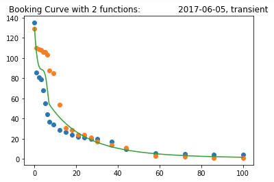
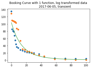
For the advance booking model, Mosaic, an innovative airline data analytics consulting firm, decided to fit a model to the booking curves themselves rather than use the past data in a lookup table, and obtained good results using log transforms of the data and piecewise estimation for various time segments. As you can see in the right chart of Figure 3, a single curve fit the booking curve fairly well except on the critical last day (when a large portion of the bookings occur). By using two separate piecewise models (left chart), the Mosaic team was able to obtain a much better fit and provide more accurate results.
Conclusion
By implementing new techniques and cutting-edge technology, Mosaic was able to significantly decrease the time required to train large and complex time-series models. In addition, by applying statistical and mathematical insight to the modeling problem, Mosaic through advanced airline data analytics consulting, added several innovations to traditional demand forecasting techniques. This provided a customized solution that was uniquely suited to the problem, and increased accuracy of forecasting for the airline industry.
- Brownlee, Jason. Machine Learning Mastery “Results from Comparing Classical and Machine Learning Methods for Time Series Forecasting,” Machine Learning Mastery, October 31, 2018, Web. 18 December 2018.
Copyright © Mosaic ATM | Airline Data Analytics Consulting. All rights reserved.
