Aviation IoT Data Mining | Problem Intro
Being a premier Aviation IoT data mining firm, we frequently encounter data mining projects. In this blog we wanted to share a recent experience of data mining that helped guide the optimization of aircraft takeoff.
We have needed to be able to predict how long a flight will take to fly its trajectory. Quite often, it has been adequate and possible to use the outputs of one of our predictive analysis tools for this purpose. It predicts both the arrival time (ETA) as well as some intermediate times that we have used in a variety of other places.
But what should we do when we can’t use our IoT data mining & predictive analysis tool? For instance, what about when we’re planning a route rather than following an existing route that the system knows about? What do we do when the system isn’t good enough? A recent project faced some of these challenges. Two of our data science consultants were able to craft a modeling solution. Despite having limited data, the resulting model turns out to be quite accurate. Typically, our model is able to predict airborne time to within one or two percent, given the route flown. On a typical two-hour flight, the model is typically within about two minutes.
Central to any such effort is the need to understand how an aircraft performs. If one has a fleet of consistently performing aircraft, one should be able to measure this correctly from our years of surveillance data. That is what we did. In a nutshell, we used historical surveillance data for one type of aircraft and atmospheric “nowcast” data from the same period, then we estimated the parameters of a performance model. Because a leading airline is our partner, and because they also happen to operate a large fleet of very similar aircraft, we chose to test the approach on their flight data.
Aviation IoT Data Mining Model Structure
Many factors affect how fast an aircraft flies, climbs and descends. Some are under the control of the operator, and in the case of an airline like our partner, some are guided by the FMS Cost Index. Most airlines adjust this according to the fuel price climate and their direct and indirect costs associated with flying an airplane. On the other hand, some factors are not under the control of the operator, such as the weather. And some are partially under the operator’s control, such as the aircraft weight.
We had hoped to gain visibility into weights, cost indices, and fuel burned for a sample of our partner’s flights, but that was not possible. So we ignored those variables, and we assumed all the flights were operated pretty much the same way. We were surprised and pleased that the result was still very good.


One can think of aircraft performance as being dictated by two things: the airplane’s performance within the air mass it’s flying through, and the movement of that air mass over the ground. One of the biggest drivers of performance of many aircraft components – wings, engines, fuselage drag – is air density. Generally, lift, drag, and related aerodynamic forces are proportional to 1/2 pv^2 (at least, within a similar operating condition, such as turbulent flow). If one can reduce air density (p) by a factor of ¼ speed (v) roughly doubles for the same amount of thrust.
That is why many airliners try to fly around 35,000 feet where the air is typically almost ¼ as dense as it is at sea level. Of course, their engines can’t produce sea-level thrust up there, but as long as the wings are big enough to keep the airplane up they don’t need to.
Because of the complexities of engine design and other parameters, to capture the performance of the aircraft through the air, we decided to estimate five parameters at different densities (Table 1). The densities we chose, by common convention, are the density in the International Standard Atmosphere (ISA) at each thousand feet of altitude up to the airplane’s operating ceiling. The ISA altitude corresponding to that density is called the density altitude and is often quite different from the geometric altitude. Thus, an aircraft that reaches 39,000 feet density altitude will have 200 parameters to be estimated (40 density altitudes times 5 parameters at each).

The second part of the model is the movement of air over the ground. Using surveillance positions (which are relative to the earth’s surface) to derive airspeed requires subtracting off the windspeed. For this effort, the source of windspeed and temperatures (needed to convert from altitude to density) was the RAP gridded numerical model, chosen largely because we could utilize historical data files for RAP corresponding to the time period of our surveillance data.
From that data, the process was conceptually simple: Take historical track data for the flights of interest (e.g., our partner B737-800’s), interpolate from the RAP gridded data to get the temperature and winds at each surveillance track point, estimate the speed over the ground at each track point, and then relate that speed over the ground into speed through the air. Next, estimate each of the 200 parameters using all of our samples generated this way. Finally, smooth the data to fit points where we don’t have many observations. For instance, 737’s seldom cruise at 15,000 feet, so that value should be smoothed to take out some of the variation due to small sample sizes.
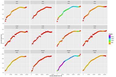
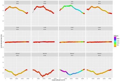
The results are shown here for the 737-300, 737-500, 737-700 and 737-800’s flown by our partner during one month in recent history.


Cruise Altitude versus Leg Length
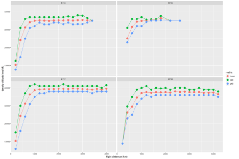
Another question to consider when building route optimization models for aviation IoT data mining is how widely to search the space of potential altitudes. Figure 3 shows the range of cruise altitudes used by 80% of the flights as a function of stage length. Shorter flights vary widely in cruise altitude, partially because some are likely stuck in the altitude restrictions of terminal airspace. They also vary because weight and weather conditions make a bigger difference in determining whether it’s worth it for a short flight to pay the cost of climbing up high for a short return on its investment. Longer flights, which eventually escape busy airspace and have plenty of time in cruise, are much more likely to fly at consistently high altitudes.

Aviation IoT Data Mining Model Evaluation
We evaluated the accuracy of the approach not only through typical goodness-of-fit measures on the parameters, but also by using them in reverse, the way one would use them in practice:
- Start with the route – in this case, we extracted the latitudes and longitudes from the track’s surveillance to get the route used historically;
- Calculate the winds estimate and density altitude at each track point through interpolation;
- Look up the appropriate parameters from the performance table and calculate the altitudes and times at each point;
- Compare the actual flight time to the time calculated by the model.
Note that there are a number of real-world reasons why actual results may differ from model results. Flow management may have been implemented to slow down the flight en route. Similarly, flights encountering turbulence prudently reduce speed. The winds aloft models are far from perfect. ATC may have restricted climb or imposed an early descent. And aircraft weights vary significantly from flight to flight, resulting in light airplanes that climb faster and achieve the higher altitudes more quickly, where they can fly faster, or heavy airplanes that do so more slowly. All these factors affect the accuracy of results.
Despite these issues, however, the median absolute errors range from less than 1% to about 1.5% of flight time (see Table 2). The 95th percentile errors were around 5% of flight time. It’s also interesting to note that the performance is quite consistent – even with only 143 flights, the B735 performance model accuracies are similar to the others.

Performance we can expect from an actual deployment of this model may differ slightly from the numbers here. First, if we have weight and cost index-type information for the flight, we can improve on these values considerably. Both have significant influence on performance and in these results, flights from the full range of cost index and weight are averaged together. In that respect then, better results can be achieved. We could get fancier still and model speed restrictions (such as for miles-in-trail) and improve them further.
On the other hand, these results were generated from the actual route flown and from the final “nowcast” of the winds aloft from RAP. To the extent that the route flown differs from the predicted route used during performance modeling, we could expect lower accuracies. And if the projection is done long enough before flight that the winds aloft were significantly different in quality from the “nowcast” winds, additional errors would be introduced.
Stay tuned for Part 2 where Mosaic uses this predictive model to build an aircraft trajectory optimization tool.
Mosaic can bring these capabilities to your organization, Contact us Here and mention this blog post.


0 Comments